Experimentation and Bayesian statistics

Overview

This guide explains the difference between frequentist and Bayesian statistics, and explains why LaunchDarkly's Experimentation framework uses Bayesian.

There are two major branches of statistics: frequentist and Bayesian. Most people don’t need to know the difference, but for the curious, this guide provides a high-level overview of the difference with respect to Experimentation. Some of the distinctions are rather technical and subtle, but here we try to highlight they key differences. This section is an introduction and is primarily focused on these two statistical methodologies in the context of Experimentation. It is not an in-depth comparison of the two.

To learn more about LaunchDarkly's Experimentation feature, read Experimentation.

To learn more about the details of the statistical methodologies used in LaunchDarkly's Experimentation feature, read Experimentation statistical methodology.

Comparison of frequentist and Bayesian statistics

In Bayesian statistics, if you collect enough data, your results will be nearly identical to your results using frequentist statistics. One way to think about this is that Bayesian statistics and frequentist statistics only differ significantly in two ways: in smaller sample sizes and in interpretation.

These are both reasons why we like Bayesian statistics for our Experimentation framework. One hurdle for a lot of experimenters is that it’s difficult to run experiments when you don’t have a large sample size. Examples of this are areas of a site with low traffic, end user types that have small populations, or business-to-business (B2B) companies. Bayesian statistics allows you to make valid inferences when those sample sizes are small, whereas often frequentist statistics will not provide statistical significance in those scenarios.

Overall, we believe that a Bayesian approach is what’s best for our customers because of its effectiveness with smaller sample sizes and its intuitive interpretation.

While frequentist experimentation can address some of the concerns discussed below, a Bayesian approach is flexible enough to work for all customers, including those who prefer the methodologies of frequentist statistics.

Frequentist and Bayesian probabilities

If you have run experiments before, you might have heard of concepts like "statistical significance" and "p-values." These are concepts from frequentist statistics. It’s called frequentist statistics because probabilities in frequentist statistics refer to the long run frequencies of a process. In other words, how a statistics method performs when repeated many, many times. For example, if you roll a 6-sided die one million times, you will roll a 1 about one in six times, a 2 about one in six times, and so on. The probability of rolling a 1 is 1/6, or 16.7%.

Bayesian statistics, on the other hand, takes probabilities to refer to our degree of belief in a particular outcome. A frequentist would say the probability of rolling a 1 on a 6-sided die is 1/6, because that’s the long-run frequency. However, a Bayesian would say the probability of rolling a 1 on a 6-sided die is that your degree of belief that it will come up 1 is 16.7%.

To understand these different interpretations of probability, the two branches of statistics use slightly different methods.

Frequentist and Bayesian modeling

So, how does it work? Bayesian statistics uses the same data as frequentist statistics, but with a slight twist. We can understand Bayesian statistics by thinking about where it shares data and statistical models with frequentist statistics.

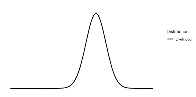
In frequentist statistics, you have some data. For simplicity, we're representing it here as a distribution called the "normal" or "Gaussian" distribution.

Here is a graph representing a normal distribution in frequentist statistics:

In frequentist statistics you use properties that we know exist over the long run for samples collected in a certain way which follow, or have parameters that follow, this distribution.

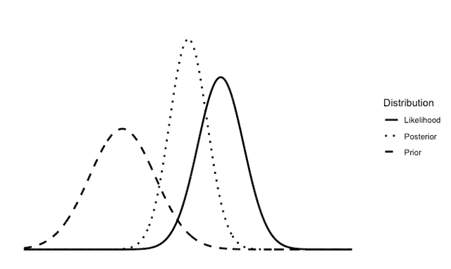
In Bayesian statistics we work with the same data. However, we also include prior beliefs we have about the data. For example, let’s suppose the data above is the heights of adult individuals in the United States. If, before collecting the data, we believe that 90% of the heights will fall between five feet and six feet, then we can start with that prior belief. After we collect the data, we can combine the data with our prior beliefs and the Bayesian updating process will provide what’s called a "posterior distribution." The posterior distribution is exactly what we should believe given our prior beliefs and the data observed.

Here is a graph representing a posterior distribution in Bayesian statistics:

Both the frequentist and Bayesian graphs use the same collected data. Bayesian statistics just incorporates prior beliefs you might have. Frequentist statistics also incorporates prior beliefs about the data, but in a very different sense. You have to pick the appropriate statistical model and process based on beliefs you have about the data, but it doesn’t incorporate prior beliefs in the same way that Bayesian does.

Frequentist and Bayesian methods

The methods and interpretations of probability for frequentist and Bayesian statistics are pretty different. For instance, because frequentist statistics is focused on long run frequencies, its foundations are around mathematical guarantees over time.

In frequentist statistics, "statistical significance" means if you ran an A/B experiment an infinite number of times, and A and B weren’t actually different, then you are guaranteed that a certain percentage of the time, your statistical test will tell you that there is a difference.

You need to specify this difference, which is the significance, or "alpha" of the test. The alpha is the the upper limit for the false positive rate, or "Type I error." If the test significance has an alpha of 5%, then it is guaranteed that your statistical test will show a significant difference of, at most, 5%, when there is no true difference. This is the null hypothesis of your test.

To be interpreted differently, Bayesian statistics requires you to specify your belief about what the outcome will be before the experiment. This is called a "prior belief." Given these prior beliefs, plus the data, Bayesian statistics can guarantee that the probabilities that it produces are exactly the degree of belief you should have.

Both methods assume that the data collection and aggregation methods are free from bias and both involve assumptions and prior beliefs, but used in different ways. Any time you choose a statistical model under either framework, you are using your prior beliefs about the data generating process. How the statistical branches use assumptions and prior beliefs is different.

Why we use Bayesian statistics

Now that you understand the differences between frequentist and Bayesian statistics, this section provides a brief overview of some of the reasons use Bayesian statistics in our experimentation platform.

Peeking

Peeking is a common problem with frequentist experimentation systems. The problem is that with traditional experimentation methods they are only valid if you analyze the data once. But this doesn’t really fit how experimenters in industry use experimentation systems. Instead, we typically want to analyze the data daily or even more frequently to see how our experiment is doing.

Some products try to prevent you from looking at the data for as long as two weeks. That works for some types of academic experiments, but if an experiment is not going well, it can be very costly to learn that too late. Other products use sequential testing within the frequentist methodology. This moves away from some of the benefits normally associated with frequentist statistics, like exact error rates, and replaces it with upper bounds on error rates.

Using Bayesian statistics, we can eliminate the peeking problem because Bayesian methods don’t have the assumption that you analyze the data exactly once. In fact, the output of the Bayesian methods we use are valid every time they’re updated, even if it is one data point at a time.

Decision making instead of error rates

In the last section, we talked about the tradeoff in frequentist statistics between allowing multiple analyses of an experiment while it’s running and having exact error rates. In our experience running and building experiments, we’ve yet to meet a customer who wants guarantees on error rates from their experimentation system. Instead, customers want to make good business decisions. This is good news for Bayesian statistics, because it doesn’t provide any guarantees on error rates. Instead, it provides you exactly the degree of belief you should have about the data. It can be combined with decision-theoretic optimal decision-making processes in a way that statistical significance can’t.

Multiple comparison problems

Another common problem we’ve had in our experience building experimentation systems at large tech companies, and one many large tech companies have talked about, is something called the "multiple comparison" problem. Just like with peeking, frequentist statistics can only guarantee error rates for a single metric in an experiment. But in industry, we typically have multiple metrics. It’s not uncommon to hear about experimentation platforms where thousands of metrics are used in a single experiment.

Some platforms allow you to apply multiple comparison corrections. However, as the number of metrics in your experiment grows, your ability to get a statistically significant result in any of them decreases. And, similar to the solution to peeking in frequentist statistics, you move away from the exact guarantees of error rates and trade it off for an upper bound.

Bayesian statistics, again, doesn’t have this problem because it doesn’t provide any guarantees on error rates. Instead, it provides the uncertainty in the measurement and what your belief ought to be, and allows you to use a decision making framework for making decisions under that uncertainty. To learn more, read Statistical Modeling, Causal Inference, and Social Science.

Interpretability

Let’s go back to the error rates mentioned above. There are two types of errors we typically think about with respect to frequentist experimentation: Type 1 errors, and Type 2 errors.

Type 1 errors are the percentage of false positives, also called statistical significance, we should expect to see over infinite experiments if there is no difference between our control and treatment. Type 2 errors are the percentage of times we’d expect to see false negatives, or no statistical significance, if there really is a difference between control and treatment.

Imagine we run an experiment and it’s statistically significant. What is the probability that it’s a false positive? We don’t know, because we don’t know if there actually is a difference or not.

If there is a difference, then there’s 0% chance that it’s a false positive. If there isn’t a difference, then there’s a 100% chance that it’s a false positive. But, we don’t know which it is.

Contrast this with Bayesian statistics. In Bayesian statistics we are given what our degree of belief should be in an outcome. This is more natural. If it tells us we should believe that treatment B has a 73% probability of being the best treatment, then that’s what we should believe.

A/B/n experiments

With traditional frequentist experimentation frameworks you are provided a p-value, or statistical significance, for each treatment as it compares to the control. This creates some difficulty in reasoning about outcomes. For instance, what if two treatments are statistically significant? Which do you choose? Or what if two treatments are very close, but one is statistically significant and the other isn’t? If your decision making framework is "choose the statistically significant treatment," it breaks down in these cases because the difference between "significant" and "not significant" is not itself statistically significant.

The Bayesian statistics we use for experimentation provides a probability for each treatment, including the control. This will allow you to choose the best treatment and use a consistent decision making framework for choosing between treatments that are close.

Status quo, or the "control"

In traditional frequentist experimentation frameworks the treatment has to "beat" the control. That is, you have to collect enough evidence to be very confident that the treatment is better than the control. This makes sense when you are developing theories and you want to falsify a particular theory. But in industry, you typically just want to know which, among a set of treatments, is best. In this case there is no reason to prefer the control in the way that frequentist methodologies do. Instead, you can reason about how much risk there is in choosing a new treatment over the status quo.

Small sample sizes

If you have small sample sizes or noisy metrics, it can be impossible to reach statistical significance. Rather than not experiment at all and not make data-driven decisions, Bayesian statistics allows you to make decisions under uncertainty by providing the uncertainty of the data and allowing you to make a decision given that uncertainty.

Conclusion

In our decades of experimentation experience both in academia and in industry, we notice that people often interpret frequentist probabilities as if they were Bayesian probabilities. For example, people say things like "the p-value is the probability that there really is a difference." Many experimentation experts have tried to correct these misinterpretations. But Bayesian statistics avails itself to this interpretation already. So instead of trying to teach unintuitive concepts, we think providing intuitive probabilities is a better approach.

You can read more details about the statistical methodology used in LaunchDarkly's Experimentation feature in Experimentation statistical methodology.